XGBoost – A Macroscopic Anatomy

XGBoost (an abbreviation of Extreme Gradient Boosting) is a machine learning package that has gained much popularity since it’s release an year back. XGBoost played the a role in the winning solutions of various data science competitions such as Avito Context Ad Click competition, Kaggle CrowdFlower Competition, WWW2015 Microsoft Malware Classification and several others.

In this blog post (which is also my first ever blog post) I will try to explain the concepts that work behind the functioning of XGBoost. I would expect my readers to know the very fundamentals of supervised learning before making an attempt to read my post.

Under The Hood

XGBoost comprises of a tree based model, i.e. a collection of decision trees. The number of trees required for a particular problem can be passed as a parameter while building the model. Mathematically the model can be represented as:

$\sum _{k=1}^k f_k$

where $f$ is a decision tree.

The prediction for the $^{i^{th}}$ data point an be written as:

$\hat{y}_i = \sum_{k=1}^k f_k(x_i)$

where $x_i$ is the feature vector of the $i^{th}$ data point.

The prediction at the $t^{th}$ step can be defined as:

$\hat{y}_{i}^{t}= \sum_{k=1}^t f_k(x_i)$

The Goal (Optimizing the loss function)

Like any other gradient descent based machine learning algorithm, the goal of XGBoost is to minimize it’s error of prediction while training. The prediction error is called loss and is calculated using a function called the loss function or cost function. XGBoost tries to optimize the three standard cost functions:

RMSE (Rooted Mean Squared Error)
- This is only used when we are trying to predict or score targets values with XGBoost. RMSE is expressed as:
  $L = \frac{1}{N}\sum_{i=1}^N (y_i - \hat{y}_i)^2$
LogLoss (Logarithmic Loss)
- Logarithmic loss is measured to check the classification error of a binary classifier. LogLoss is the measure of cross entropy and acts as a soft measurement of accuracy. By minimizing cross entropy we can maximize the accuracy of a classifier. LogLoss cost function is expressed as: $L = -\frac{1}{N}\sum_{i=1}^N (y_i log(p_i)) + (1 - y_i) log(1 - p_i))$
  where $p_i$ is the prediction
mLogLoss (Multiclass Logarithmic Loss)
- This is used to measure the prediction loss of a multi class classifier and is essentially a generalized version of LogLoss which is used only for binary classifiers. The mLogLoss function is expressed as:
  $L = -\frac{1}{N}\sum_{i=1}^N\sum_{j=1}^M y_{i,j} log(p_{i,j})$

Preventing Learning by Heart (Regularization)

While optimizing the objective is our primary goal, that’s not the only thing that we should keep in mind while training a machine learning model. During training it is often the case where the model learns the training data by heart and fails to predict the target of any new data point. In other words the model builds intricate structures (or equations) within itself that can correctly predict the target for all (or most) of the data points in the training set but will fail when tested with “unseen” data. Think of this as connecting three collinear dots with an ‘S’ like curve instead of maybe a straight line. This problem is known as overfitting.

In order to make the model more generalized, we need to “relax” the model a bit in each training step, this process is called regularization. In order to prevent a model from over complicating itself, we must first define the model complexity. The complexity of XGBoost can be represented as:

$\Omega = \gamma T + \frac{1}{2} \lambda \sum_{j=1}^T w_j^2$

Where $T$ is the number of leaves and $w_j$ is the score on the $j^{th}$ leaf. $\gamma$ and $\lambda$ are constants which can be passed as parameters while building the model and are used to tune the degree of regularization or relaxation.

Now that we have our cost function and complexity of the model defined, lets use them to redefine our goal:

$Goal = L + \Omega$

Towards The Goal (Gradient Descent)

Gradient descent is the chosen algorithm by XGBoost to optimize it’s goal or objective function. Let’s first define gradient descent:

Given an objective $Goal(y, \hat{y})$ , for each iteration, the partial derivative $\partial_{\hat{y}} Goal(y, \hat{y})$ is calculated. Then $\hat{y}$ is improved along the direction of the gradient to minimize the objective. This process continues till there can be no further improvements i.e. till the global optima is reached (convergence).

For the gradient descent in XGBoost, the objective function that needs to be differentiated in the $t^{th}$ step is:

$Goal^{(t)} = \sum_{i = 1}^N L (y_i, \hat{y_i}^t) + \sum_{i = 1}^t \Omega (f_i)$

But we need not calculate $L (y_i, \hat{y_i}^{(t)})$ at every step if we store the value of the loss function in the previous step. The equation then becomes:

$Goal^{(t)} = \sum_{i = 1}^N L (y_i, \hat{y_i}^{(t - 1)} + f_t (x_i)) + \sum_{i = 1}^t \Omega (f_i)$

The performance of gradient descent can be further improved if we consider both the first and the second order gradient of the objective function. Thus is in each step we should calculate:

$\partial_{\hat{y_i}^{(t)}} (Goal^{(t)})$
$\partial_{\hat{y_i}^{(t)}}^2 (Goal^{(t)})$

This will lead to faster convergence as the second order derivative gives us a proper approximation of the direction of descent in each step.

Since derivatives of all functions can’t be calculated, we have to calculate the second order Taylor’s approximation of the derivative. Our objective function now becomes:

$Goal^{(t)} \simeq \sum_{i = 1}^N [L (y_i, \hat{y^{t - 1}}) + g_i f_t (x_i) + \frac{1}{2} h_i f_t^2 (x_i)] + \sum_{i = 1}^t \Omega (f_i)$

where:

$g_i = \partial_{\hat{y}^{(t - 1)}} l (y_i, \hat{y}^{(t - 1)})$ is the first order gradient and
$h_i = \partial_{\hat{y}^{(t - 1)}}^2 l (y_i, \hat{y}^{(t - 1)})$ is the second order gradient of the cost function.

Now since $L(y_i, \hat{y}^{(t - 1)})$ becomes a constant, our objective at the $t^{th}$ step boils down to:

$Goal^{(t)} \simeq \sum_{i = 1}^N [g_i f_t (x_i) + \frac{1}{2} h_i f_t^2 (x_i)] + \sum_{i = 1}^t \Omega (f_i)$

All that remains now is to find a proper $f_t$ to optimize it.

The Hurdles Along the Way

As easy as it sounds, finding a $f_t$ that optimizes a tree based model is not so trivial. Let’s state the problem of finding $f_t$ in another way:

“How do we find a decision tree that improves it’s prediction along the gradient?”

XGBoost has a very clever implementation of the solution, but before diving in let’s first understand the concepts that are used:

Internal Nodes

Each internal node splits the flow of data points by using one feature from the feature space.
Each node selects a threshold value from a feature and based upon some conditions on that threshold, specifies the direction of the flow of data (either left child node or the right child node).

Leaves

The flow of data end at leaves. The leaves are assigned a weight.
The weight of a leaf corresponds to the leaves prediction.

This, as you might have realized is the basic of any CART (Classification and Regression Tree) building algorithm, but the devil lies in the details. The two key questions XGBoost addresses are:

How to assign prediction score to the leaves?
How to find a proper tree structure?

Let us know try to understand how XGBoost answers these two questions.

Assigning weights to the leaves

Mathematically, a tree can be represented as:

$f_t (x) = w_q (x)$

where $q(x)$ is a “directing” function which assigns every data point to the $q(x)^{th}$ leaf.

With this definition of a tree, we can describe the weight assigning process as:

Assign the data point $x$ to a leaf by $q$ .
Assign the corresponding score $w_q(x)$ on the $q(x)^{(th)}$ leaf to the data point.

Where $q(x)$ is the leaf index and the index set is defined as set of indices of the data points that are assigned to the $j^{th}$ leaf. We can write the index set as:

$I_j = \{i | q (x_i) = j\}$

The objective function can (again) be re-written as:

$Goal^{(t)} = \sum_{i = 1}^N [g_i f_t (x_i) + \frac{1}{2} h_i f_t^2 (x_i)] + \gamma T + \frac{1}{2} \lambda \sum_{j = 1}^T w_j^2$

where $N$ is the number of data points, but instead of writing the objective function as a summation of separate data points, we can write it in a fashion where we consider the summation of leaf weights. Thus the new representation becomes:

$Goal^{(t)} = \sum_{j = 1}^T [(\sum_{i \in I_j}) w_j + \frac{1}{2} (\sum_{i \in I_j} h_i + \lambda) w_j^2] + \gamma T$

(Since all the data points on the same leaf share the same prediction)

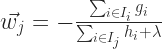
As you might have noticed, the above equation is a equation is a quadratic equation of $w_j$ . All that remains now is to find a solution to the quadratic equation to get a $\vec{w}$ vector which will optimize the objective. The solution is very simply:

$\vec{w_j} = - \frac{\sum_{i \in I_i} g_i}{\sum_{i \in I_j} h_i + \lambda}$

Then the corresponding value of $Goal$ becomes:

$Goal^{(t)} = - \frac{1}{2} \sum_{j = 1}^T \frac{(\sum_{i \in I_j} g_i)^2}{\sum_{i \in I_j} h_i + \lambda} + \gamma T$

Finding the proper tree structure

The algorithm to find a proper tree structure is in each split, the best splitting point is found that can optimize the objective. This is implemented as-

For each feature:

Sort the numbers.
Scan the best splitting point (more on this in the next section)
Choose the best feature.

Now let us try to understand the definition of “Best Split”:

Every time a split is made, a leaf node gets converted to an internal node. If a particular split improves the objective function, the gain for the split is positive, but if the split degrades the model, the gain is negative. So how do we calculate gain?

Let:

$I$ be the set of indices of data points assigned to a node.
$I_L$ and $I_R$ be the set of indices of data points assigned to the new left and right leaves respectively

So the gain becomes:

$gain = \frac{1}{2} [Goal(leaf_{left}) + Goal(leaf_{right}) - Goal(parent)] - \gamma$

$OR$

$gain = \frac{1}{2} [\frac{(\sum_{i \in I_L} g_i)^2}{\sum_{i \in I_L} h_i + \lambda} + \frac{(\sum_{i \in I_R} g_i)^2}{\sum_{i \in I_R} h_i + \lambda} - \frac{(\sum_{i \in I} g_i)^2}{\sum_{i \in I} h_i + \lambda}] - \gamma$

While building a tree, the best splitting point is found until the max depth (supplied as a parameter) is reached. The nodes with negative gain are deleted by pruning the tree in a bottom up manner. The intuition behind this is that it is okay to have a node with negative gain in the middle of the tree as the gain the might increase significantly down it’s child nodes.

Note that this is an unique feature of XGBoost as traditionally, gain is measured by calculating Gini coefficient or by entropy matrix.

The Big Question (How to handle missing values)

The most unique feature of XGBoost is it’s inherent ability to handle missing values. For any kind of data set, handling missing values is always a challenge. There are both statistical and machine learning processes to impute missing values in a data set, but XGBoost avoids any such method all together. I will now make an attempt to describe how XGBoost handles missing values.

For each node, all the data points with missing values are:

Put to the left child node and the maximum gain is calculated.
Then they are put to the right child node and the maximum gain is calculated.
The direction with larger gain is chosen.

Hence every node has a default direction for missing values.

Gist

To sum it up in a few lines, the work flow of XGboost is:

For $n_{round}$ times do:

Grow the tree to the maximum possible dept.

Find the best splitting point.
Assign weights to the leaves.

Prune the tree from bottom up to delete nodes with negative gain.

8 Comments

Add yours →

Rohan Rao November 14, 2015 — 5:27 pm

Excellent read. Very nice capstone of XGBoost.

LikeLike

Aarshay Jain February 19, 2016 — 6:42 am

Very nice article. I really like the mathematical concepts explained. I have a question – how do we define the ‘gamma’ and ‘lambda’ for regularization in a classification problem? There is a parameter ‘gamma’ which is the minimum loss reduction required for a split. Is it related to the gamma in regularization? What bout lambda?

LikeLike

Aarshay Jain February 19, 2016 — 6:45 am

Very nice article, specially the mathematical context.

I have a question – How do we define regularization parameters ‘lambda’ and ‘gamma’ for classification?

I am using Python version of xgboost and I see a parameter ‘gamma’ which is the minimum loss reduction required for a split. Is it related to the regularization?

Also, the parameters ‘lambda’ and ‘alpha’ are only for linear booster.

LikeLike

- (Post author)
  
  nilabhraroy February 19, 2016 — 9:19 am
  
  Thanks, glad you liked it.
  
  You can set the values of the parameters lambda and gamma for both tree boosting and also for linear boosting. In both the cases lamda is the L2 regularization term, and alpha is of L1. You can decide what to use depending on the data. Gamma is used to determine if a split would be made on a leaf. Larger the value of gamma, more conservative the tree would be. Personally I would not touch gamma unless I have to.
  
  Hope this answers your query. You can find more info on XGBOOST parameters at:
  http://xgboost.readthedocs.org/en/latest/parameter.html
  
  For a indepth understanding of regularization check my other blog post:
  https://chaoticsenses.wordpress.com/2016/01/20/taming-the-beast-with-regularization-3/
  
  LikeLike
  
  - Aarshay Jain February 19, 2016 — 9:57 am
    
    Thanks for your response.
    I was just looking up xgboost implementation in Python. What’s the difference between ‘eta’ parameters in the params and the learning_rates argument in the train function?
    
    LikeLike
(Post author)

nilabhraroy February 19, 2016 — 1:00 pm

I am not aware of the learning_rate parameter, I always use eta to define learning rate of the model. I’ll get back if I find anything.

LikeLike

- Aarshay Jain February 19, 2016 — 1:03 pm
  
  sure thanks..
  
  LikeLike
  
Patrick March 4, 2016 — 10:08 pm

Learning_rate and eta are identical… it just depends on if you are using native xgboost or the python wrapper. If you’re code looks like XGBClassifier(_params_) and you can call ‘.fit’, that is the wrapper and you should use learning_rate. If you are using ‘.train’ use eta.

LikeLike

	Patrick on XGBoost – A Macroscopic…
	Aarshay Jain on XGBoost – A Macroscopic…
	nilabhraroy on XGBoost – A Macroscopic…
	Aarshay Jain on XGBoost – A Macroscopic…
	nilabhraroy on XGBoost – A Macroscopic…

Chaotic Senses